Zero-inflated Poisson distributions are frequently used to model counts with many zero observations.
Details
We recommend reading this documentation on https://alexpghayes.github.io/distributions3/, where the math will render with additional detail.
In the following, let \(X\) be a zero-inflated Poisson random variable with parameter
lambda = \(\lambda\).
Support: \(\{0, 1, 2, 3, ...\}\)
Mean: \((1 - \pi) \cdot \lambda\)
Variance: \((1 - \pi) \cdot \lambda \cdot (1 + \pi \cdot \lambda)\)
Probability mass function (p.m.f.):
$$ P(X = k) = \pi \cdot I_{0}(k) + (1 - \pi) \cdot f(k; \lambda) $$
where \(I_{0}(k)\) is the indicator function for zero and
\(f(k; \lambda)\) is the p.m.f. of the Poisson
distribution.
Cumulative distribution function (c.d.f.):
$$ P(X \le k) = \pi + (1 - \pi) \cdot F(k; \lambda) $$
where \(F(k; \lambda)\) is the c.d.f. of the Poisson distribution.
Moment generating function (m.g.f.):
$$ E(e^{tX}) = \pi + (1 - \pi) \cdot e^{\lambda (e^t - 1)} $$
See also
Other discrete distributions:
Bernoulli(),
Binomial(),
Categorical(),
Geometric(),
HurdleNegativeBinomial(),
HurdlePoisson(),
HyperGeometric(),
Multinomial(),
NegativeBinomial(),
Poisson(),
PoissonBinomial(),
ZINegativeBinomial(),
ZTNegativeBinomial(),
ZTPoisson()
Examples
## set up a zero-inflated Poisson distribution
X <- ZIPoisson(lambda = 2.5, pi = 0.25)
X
#> [1] "ZIPoisson(lambda = 2.5, pi = 0.25)"
## standard functions
pdf(X, 0:8)
#> [1] 0.311563749 0.153909372 0.192386716 0.160322263 0.100201414 0.050100707
#> [7] 0.020875295 0.007455462 0.002329832
cdf(X, 0:8)
#> [1] 0.3115637 0.4654731 0.6578598 0.8181821 0.9183835 0.9684842 0.9893595
#> [8] 0.9968150 0.9991448
quantile(X, seq(0, 1, by = 0.25))
#> [1] 0 0 2 3 Inf
## cdf() and quantile() are inverses for each other
quantile(X, cdf(X, 3))
#> [1] 3
## density visualization
plot(0:8, pdf(X, 0:8), type = "h", lwd = 2)
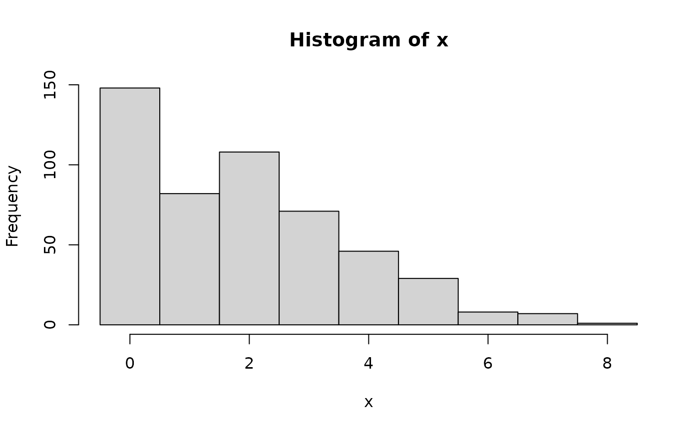
 ## corresponding sample with histogram of empirical frequencies
set.seed(0)
x <- random(X, 500)
hist(x, breaks = -1:max(x) + 0.5)
## corresponding sample with histogram of empirical frequencies
set.seed(0)
x <- random(X, 500)
hist(x, breaks = -1:max(x) + 0.5)