Two sample Z-tests

In this vignette, we work through a two sample Z-test. If you haven’t seen a one-sample Z-test, we recommend you read vignette("one-sample-z-test") first.

Problem setup

Let’s suppose that a student wants to figure out if biology professors or English professors know more memes. The student writes a meme quiz and springs it on 14 unsuspecting biology professors and 18 unsuspecting English professors during office hours.

The biology professors get the following scores:

$$3, 7, 11, 0, 7, 0, 4, 5, 6, 2, 4, 7, 2, 9$$

and the English professors score:

$$5, 5, 4, 5, 4, 5, 7, 2, 6, 2, 2, 7, 2, 6, 4, 2, 5, 2$$

We’ll assume that the population variance of the biology professor scores is $\sigma^2_1 = 3$ and the population variance of the English professor scores is $\sigma^2_2 = 2$.

Assumption checking

Before we can do a Z-test, we need to make check if we can reasonably treat the means of each sample as normally distributed. This happens is the case of either of following hold:

1. The data comes from a normal distribution.
2. We have lots of data. How much? Many textbooks use 30 data points as a rule of thumb.

Since both of samples have less than 30 data points, we need to check if they are plausibly from normal distributions. We check the biology professor scores first using a normal quantile-quantile plot.

biology <- c(3, 7, 11, 0, 7, 0, 4, 5, 6, 2, 4, 7, 2, 9)
english <- c(8, 5, 4, 10, 4, 5, 7, 2, 6, 1, 2, 7, 0, 6, 4, 12, 5, 2)

qqnorm(biology)
qqline(biology)

Since the biology scores lies close the line $y = x$, and has no notable systematic deviations from line, it’s safe to treat the sample as coming from a normal distribution. Honestly this quantile-quantile plot is so good it’s suspicious.

Anyway, next we check the English scores

qqnorm(english)
qqline(english)

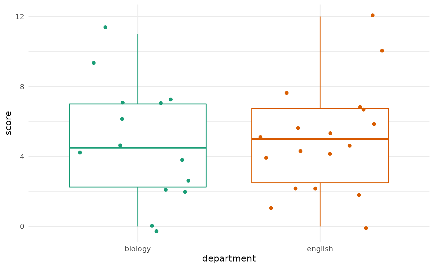
And it seems fine as well. We can also create side-by-side boxplots of the data using the ggplot2 package to get a nice comparison of the two groups. This requires a little bit of data manipulation:

library(ggplot2)

# make a data frame in long format for plotting
test_results <- data.frame(
  score = c(biology, english),
  department = c(
    rep("biology", length(biology)),
    rep("english", length(english))
  )
)

ggplot(test_results, aes(x = department, y = score, color = department)) +
  geom_boxplot() +
  geom_jitter() +
  scale_color_brewer(type = "qual", palette = 2) +
  theme_minimal() +
  theme(legend.position = "none")

Based on eye-balling the data, we’d be pretty surprised if we rejected a null hypothesis of equal means between the two groups.

Null hypothesis and test statistic

Let’s write the null hypothesis out (here we treat biology professors as group 1 and English professors as group 2):

$$H_0: \mu_1 - \mu_2 = 0 \qquad H_A: \mu_1 - \mu_2 \neq 0$$

First we need to calculate our Z-statistic. Let’s use do this with R. Remember that the Z-statistic is defined as

$$Z = \frac{\bar x_1 - \bar x_2 - \delta_0} {\sqrt{\sigma_1^2 / n_1 + \sigma_2^2 / n_2}} \sim \mathrm{Normal}(0, 1)$$

In R this looks like:

delta_0 <- 0

# by assumption
sigma_sq_1 <- 3
sigma_sq_2 <- 2

n_1 <- length(biology)
n_2 <- length(english)

# calculate the z-statistic
z_stat <- (mean(biology) - mean(english) - delta_0) / 
  sqrt(sigma_sq_1 / n_1 + sigma_sq_2 / n_2)

z_stat
#> [1] -0.3756527

Calculating p-values

To calculate a two-sided p-value, we need to find

$$\begin{align} P(|Z| \ge |-0.376|) &= P(Z \ge 0.376) + P(Z \le -0.376) \\ &= 1 - P(Z \le 0.376) + P(Z \le -0.376) \\ &= 1 - \Phi(0.376) + \Phi(0.376) \end{align}$$

To do this we need to c.d.f. of a standard normal

library(distributions3)

Z <- Normal(0, 1)  # make a standard normal r.v.
1 - cdf(Z, 0.376) + cdf(Z, -0.376)
#> [1] 0.7069169

Note that we saved z_stat above so we could have also done

1 - cdf(Z, abs(z_stat)) + cdf(Z, -abs(z_stat))
#> [1] 0.7071751

which is slightly more accurate since there is no rounding error.

So our p-value is about 0.71. You should verify this with a Z-table. Note that you should get the same value from cdf(Z, -0.376) and looking up -0.376 on a Z-table.

You may also have seen a different formula for the p-value of a two-sided Z-test, which makes use of the fact that the normal distribution is symmetric:

$$\begin{align} P(|Z| \ge |-0.376|) &= 2 \cdot P(Z \le -|-0.376|) &= 2 \cdot \Phi(-0.376) \end{align}$$

Using this formula we get the same result:

2 * cdf(Z, -0.376)
#> [1] 0.7069169

Finally, sometimes we are interest in one sided Z-tests. For the test

$$\begin{align} H_0: \mu \le 3 \qquad H_A: \mu > 3 \end{align}$$

the p-value is given by

$$P(Z > -0.376)$$

which we calculate with

1 - cdf(Z, -0.376)
#> [1] 0.6465416

For the test

$$H_0: \mu \ge 3 \qquad H_A: \mu < 3$$

the p-value is given by

$$P(Z < -0.376)$$

which we calculate with

cdf(Z, -0.376)
#> [1] 0.3534584