The zero-inflated negative binomial distribution

Density, distribution function, quantile function, and random generation for the zero-inflated negative binomial distribution with parameters mu, theta (or size), and pi.

Usage

dzinbinom(x, mu, theta, size, pi, log = FALSE)

pzinbinom(q, mu, theta, size, pi, lower.tail = TRUE, log.p = FALSE)

qzinbinom(p, mu, theta, size, pi, lower.tail = TRUE, log.p = FALSE)

rzinbinom(n, mu, theta, size, pi)

Arguments

x

vector of (non-negative integer) quantiles.

mu

vector of (non-negative) negative binomial location parameters.

theta, size

vector of (non-negative) negative binomial overdispersion parameters. Only theta or, equivalently, size may be specified.

pi

vector of zero-inflation probabilities in the unit interval.

log, log.p

logical indicating whether probabilities p are given as log(p).

q

vector of quantiles.

lower.tail

logical indicating whether probabilities are \(P[X \le x]\) (lower tail) or \(P[X > x]\) (upper tail).

p

vector of probabilities.

n

number of random values to return.

Details

All functions follow the usual conventions of d/p/q/r functions in base R. In particular, all four zinbinom functions for the zero-inflated negative binomial distribution call the corresponding nbinom functions for the negative binomial distribution from base R internally.

Note, however, that the precision of qzinbinom for very large probabilities (close to 1) is limited because the probabilities are internally handled in levels and not in logs (even if log.p = TRUE).

See also

ZINegativeBinomial, dnbinom

Examples

## theoretical probabilities for a zero-inflated negative binomial distribution
x <- 0:8
p <- dzinbinom(x, mu = 2.5, theta = 1, pi = 0.25)
plot(x, p, type = "h", lwd = 2)


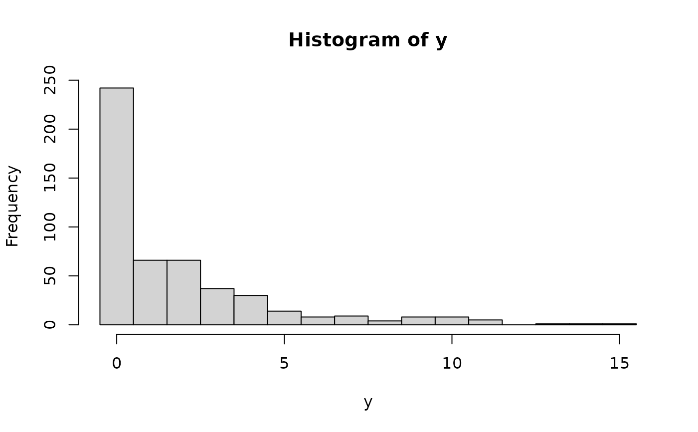
## corresponding empirical frequencies from a simulated sample
set.seed(0)
y <- rzinbinom(500, mu = 2.5, theta = 1, pi = 0.25)
hist(y, breaks = -1:max(y) + 0.5)