Determine quantiles of a zero-truncated Poisson distribution

quantile() is the inverse of cdf().

Usage

# S3 method for ZTPoisson
quantile(x, probs, drop = TRUE, elementwise = NULL, ...)

Arguments

x

A ZTPoisson object created by a call to ZTPoisson().

probs

A vector of probabilities.

drop

logical. Should the result be simplified to a vector if possible?

elementwise

logical. Should each distribution in x be evaluated at all elements of probs (elementwise = FALSE, yielding a matrix)? Or, if x and probs have the same length, should the evaluation be done element by element (elementwise = TRUE, yielding a vector)? The default of NULL means that elementwise = TRUE is used if the lengths match and otherwise elementwise = FALSE is used.

...

Arguments to be passed to qztpois. Unevaluated arguments will generate a warning to catch mispellings or other possible errors.

Value

In case of a single distribution object, either a numeric vector of length probs (if drop = TRUE, default) or a matrix with length(probs) columns (if drop = FALSE). In case of a vectorized distribution object, a matrix with length(probs) columns containing all possible combinations.

Examples

## set up a zero-truncated Poisson distribution
X <- ZTPoisson(lambda = 2.5)
X
#> [1] "ZTPoisson distribution (lambda = 2.5)"

## standard functions
pdf(X, 0:8)
#> [1] 0.000000000 0.223563725 0.279454656 0.232878880 0.145549300 0.072774650
#> [7] 0.030322771 0.010829561 0.003384238
cdf(X, 0:8)
#> [1] 0.0000000 0.2235637 0.5030184 0.7358973 0.8814466 0.9542212 0.9845440
#> [8] 0.9953735 0.9987578
quantile(X, seq(0, 1, by = 0.25))
#> [1]   1   2   2   4 Inf

## cdf() and quantile() are inverses for each other
quantile(X, cdf(X, 3))
#> [1] 3

## density visualization
plot(0:8, pdf(X, 0:8), type = "h", lwd = 2)


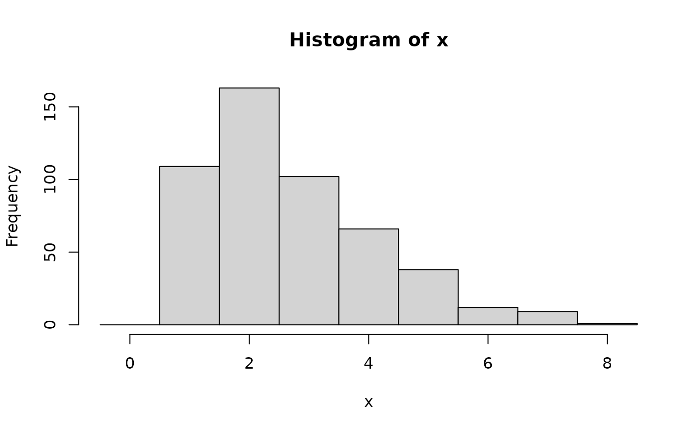
## corresponding sample with histogram of empirical frequencies
set.seed(0)
x <- random(X, 500)
hist(x, breaks = -1:max(x) + 0.5)