Determine quantiles of a zero-truncated negative binomial distribution
Source:R/ZTNegativeBinomial.R
quantile.ZTNegativeBinomial.Rdquantile() is the inverse of cdf().
Usage
# S3 method for class 'ZTNegativeBinomial'
quantile(x, probs, drop = TRUE, elementwise = NULL, ...)
Arguments
- x
A
ZTNegativeBinomialobject created by a call toZTNegativeBinomial().- probs
A vector of probabilities.
- drop
logical. Should the result be simplified to a vector if possible?
- elementwise
logical. Should each distribution in
xbe evaluated at all elements ofprobs(elementwise = FALSE, yielding a matrix)? Or, ifxandprobshave the same length, should the evaluation be done element by element (elementwise = TRUE, yielding a vector)? The default ofNULLmeans thatelementwise = TRUEis used if the lengths match and otherwiseelementwise = FALSEis used.- ...
Arguments to be passed to
qztnbinom. Unevaluated arguments will generate a warning to catch mispellings or other possible errors.
Value
In case of a single distribution object, either a numeric
vector of length probs (if drop = TRUE, default) or a matrix with
length(probs) columns (if drop = FALSE). In case of a vectorized
distribution object, a matrix with length(probs) columns containing all
possible combinations.
Examples
## set up a zero-truncated negative binomial distribution
X <- ZTNegativeBinomial(mu = 2.5, theta = 1)
X
#> [1] "ZTNegativeBinomial(mu = 2.5, theta = 1)"
## standard functions
pdf(X, 0:8)
#> [1] 0.00000000 0.28571429 0.20408163 0.14577259 0.10412328 0.07437377 0.05312412
#> [8] 0.03794580 0.02710414
cdf(X, 0:8)
#> [1] 0.0000000 0.2857143 0.4897959 0.6355685 0.7396918 0.8140656 0.8671897
#> [8] 0.9051355 0.9322396
quantile(X, seq(0, 1, by = 0.25))
#> [1] 1 1 3 5 Inf
## cdf() and quantile() are inverses for each other
quantile(X, cdf(X, 3))
#> [1] 3
## density visualization
plot(0:8, pdf(X, 0:8), type = "h", lwd = 2)
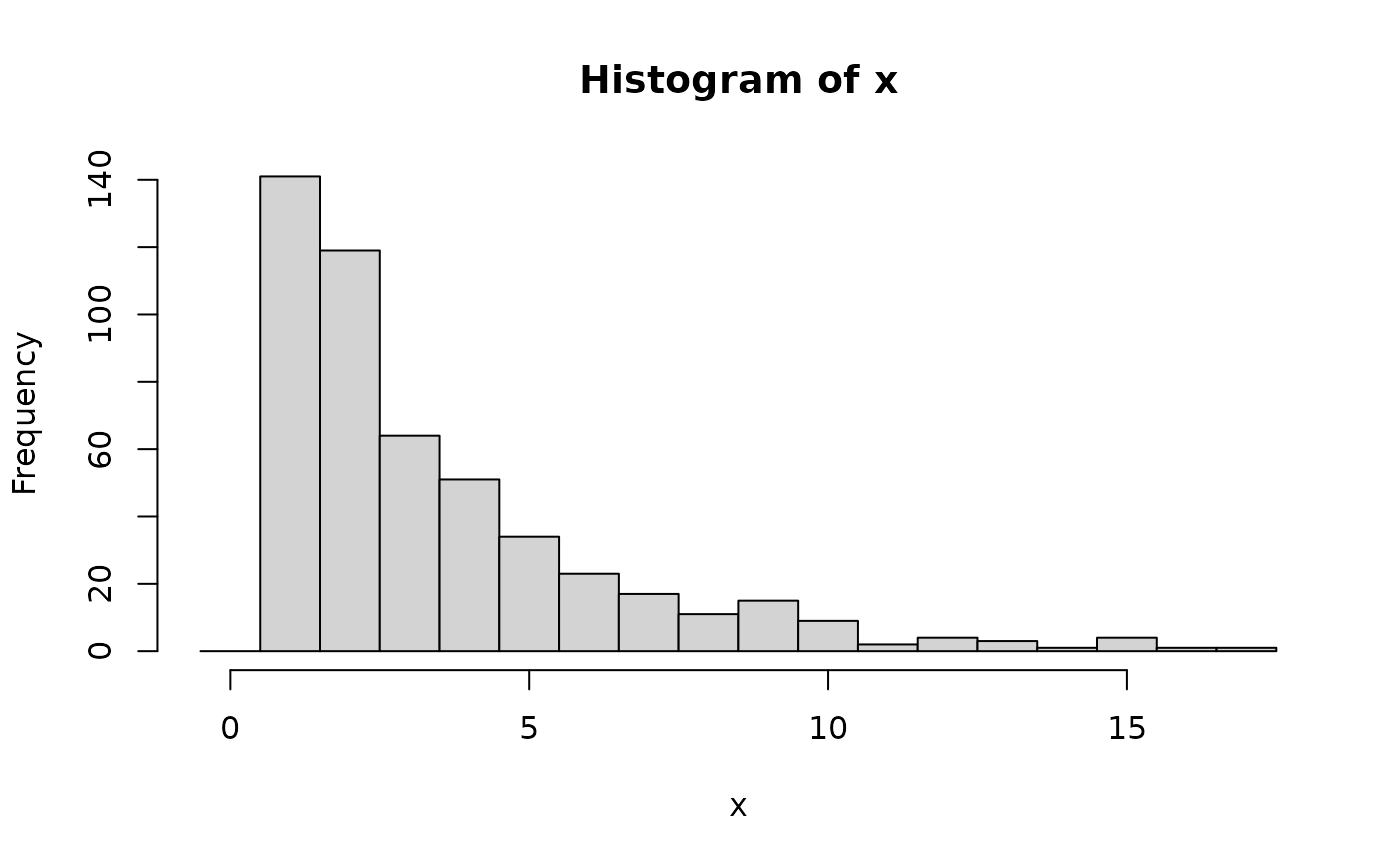
 ## corresponding sample with histogram of empirical frequencies
set.seed(0)
x <- random(X, 500)
hist(x, breaks = -1:max(x) + 0.5)
## corresponding sample with histogram of empirical frequencies
set.seed(0)
x <- random(X, 500)
hist(x, breaks = -1:max(x) + 0.5)