Determine quantiles of a hurdle Poisson distribution
Source:R/HurdlePoisson.R
quantile.HurdlePoisson.Rdquantile() is the inverse of cdf().
Usage
# S3 method for class 'HurdlePoisson'
quantile(x, probs, drop = TRUE, elementwise = NULL, ...)
Arguments
- x
A
HurdlePoissonobject created by a call toHurdlePoisson().- probs
A vector of probabilities.
- drop
logical. Should the result be simplified to a vector if possible?
- elementwise
logical. Should each distribution in
xbe evaluated at all elements ofprobs(elementwise = FALSE, yielding a matrix)? Or, ifxandprobshave the same length, should the evaluation be done element by element (elementwise = TRUE, yielding a vector)? The default ofNULLmeans thatelementwise = TRUEis used if the lengths match and otherwiseelementwise = FALSEis used.- ...
Arguments to be passed to
qhpois. Unevaluated arguments will generate a warning to catch mispellings or other possible errors.
Value
In case of a single distribution object, either a numeric
vector of length probs (if drop = TRUE, default) or a matrix with
length(probs) columns (if drop = FALSE). In case of a vectorized
distribution object, a matrix with length(probs) columns containing all
possible combinations.
Examples
## set up a hurdle Poisson distribution
X <- HurdlePoisson(lambda = 2.5, pi = 0.75)
X
#> [1] "HurdlePoisson(lambda = 2.5, pi = 0.75)"
## standard functions
pdf(X, 0:8)
#> [1] 0.250000000 0.167672793 0.209590992 0.174659160 0.109161975 0.054580987
#> [7] 0.022742078 0.008122171 0.002538178
cdf(X, 0:8)
#> [1] 0.2500000 0.4176728 0.6272638 0.8019229 0.9110849 0.9656659 0.9884080
#> [8] 0.9965302 0.9990683
quantile(X, seq(0, 1, by = 0.25))
#> [1] 0 0 2 3 Inf
## cdf() and quantile() are inverses for each other
quantile(X, cdf(X, 3))
#> [1] 3
## density visualization
plot(0:8, pdf(X, 0:8), type = "h", lwd = 2)
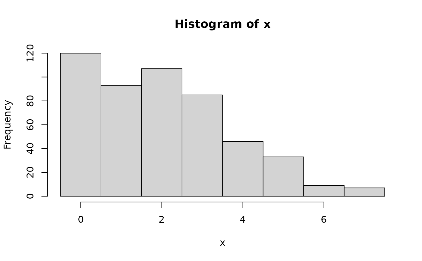
 ## corresponding sample with histogram of empirical frequencies
set.seed(0)
x <- random(X, 500)
hist(x, breaks = -1:max(x) + 0.5)
## corresponding sample with histogram of empirical frequencies
set.seed(0)
x <- random(X, 500)
hist(x, breaks = -1:max(x) + 0.5)