Determine quantiles of a zero-inflated negative binomial distribution

quantile() is the inverse of cdf().

Usage

# S3 method for class 'ZINegativeBinomial'
quantile(x, probs, drop = TRUE, elementwise = NULL, ...)

Arguments

x

A ZINegativeBinomial object created by a call to ZINegativeBinomial().

probs

A vector of probabilities.

drop

logical. Should the result be simplified to a vector if possible?

elementwise

logical. Should each distribution in x be evaluated at all elements of probs (elementwise = FALSE, yielding a matrix)? Or, if x and probs have the same length, should the evaluation be done element by element (elementwise = TRUE, yielding a vector)? The default of NULL means that elementwise = TRUE is used if the lengths match and otherwise elementwise = FALSE is used.

...

Arguments to be passed to qzinbinom. Unevaluated arguments will generate a warning to catch mispellings or other possible errors.

Value

In case of a single distribution object, either a numeric vector of length probs (if drop = TRUE, default) or a matrix with length(probs) columns (if drop = FALSE). In case of a vectorized distribution object, a matrix with length(probs) columns containing all possible combinations.

Examples

## set up a zero-inflated negative binomial distribution
X <- ZINegativeBinomial(mu = 2.5, theta = 1, pi = 0.25)
X
#> [1] "ZINegativeBinomial(mu = 2.5, theta = 1, pi = 0.25)"

## standard functions
pdf(X, 0:8)
#> [1] 0.46428571 0.15306122 0.10932945 0.07809246 0.05578033 0.03984309 0.02845935
#> [8] 0.02032811 0.01452008
cdf(X, 0:8)
#> [1] 0.4642857 0.6173469 0.7266764 0.8047688 0.8605492 0.9003923 0.9288516
#> [8] 0.9491797 0.9636998
quantile(X, seq(0, 1, by = 0.25))
#> [1]   0   0   1   3 Inf

## cdf() and quantile() are inverses for each other
quantile(X, cdf(X, 3))
#> [1] 3

## density visualization
plot(0:8, pdf(X, 0:8), type = "h", lwd = 2)


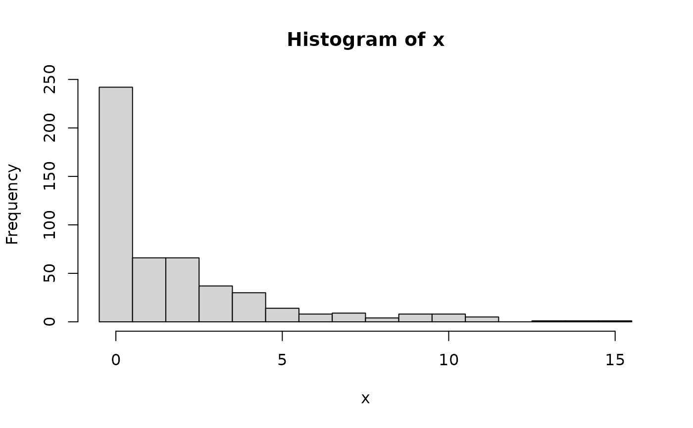
## corresponding sample with histogram of empirical frequencies
set.seed(0)
x <- random(X, 500)
hist(x, breaks = -1:max(x) + 0.5)