Evaluate the cumulative distribution function of a zero-inflated Poisson distribution

Usage

# S3 method for ZIPoisson
cdf(d, x, drop = TRUE, elementwise = NULL, ...)

Arguments

d: A ZIPoisson object created by a call to ZIPoisson().
x: A vector of elements whose cumulative probabilities you would like to determine given the distribution d.
drop: logical. Should the result be simplified to a vector if possible?
elementwise: logical. Should each distribution in d be evaluated at all elements of x (elementwise = FALSE, yielding a matrix)? Or, if d and x have the same length, should the evaluation be done element by element (elementwise = TRUE, yielding a vector)? The default of NULL means that elementwise = TRUE is used if the lengths match and otherwise elementwise = FALSE is used.
...: Arguments to be passed to pzipois. Unevaluated arguments will generate a warning to catch mispellings or other possible errors.

Value

In case of a single distribution object, either a numeric vector of length probs (if drop = TRUE, default) or a matrix with length(x) columns (if drop = FALSE). In case of a vectorized distribution object, a matrix with length(x) columns containing all possible combinations.

Examples

## set up a zero-inflated Poisson distribution
X <- ZIPoisson(lambda = 2.5, pi = 0.25)
X
#> [1] "ZIPoisson distribution (lambda = 2.5, pi = 0.25)"

## standard functions
pdf(X, 0:8)
#> [1] 0.311563749 0.153909372 0.192386716 0.160322263 0.100201414 0.050100707
#> [7] 0.020875295 0.007455462 0.002329832
cdf(X, 0:8)
#> [1] 0.3115637 0.4654731 0.6578598 0.8181821 0.9183835 0.9684842 0.9893595
#> [8] 0.9968150 0.9991448
quantile(X, seq(0, 1, by = 0.25))
#> [1]   0   0   2   3 Inf

## cdf() and quantile() are inverses for each other
quantile(X, cdf(X, 3))
#> [1] 3

## density visualization
plot(0:8, pdf(X, 0:8), type = "h", lwd = 2)


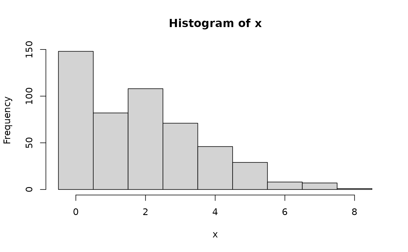
## corresponding sample with histogram of empirical frequencies
set.seed(0)
x <- random(X, 500)
hist(x, breaks = -1:max(x) + 0.5)