Create a zero-truncated negative binomial distribution
Source:R/ZTNegativeBinomial.R
ZTNegativeBinomial.RdZero-truncated negative binomial distributions are frequently used to model counts where zero observations cannot occur or have been excluded.
Details
We recommend reading this documentation on https://alexpghayes.github.io/distributions3/, where the math will render with additional detail.
In the following, let \(X\) be a zero-truncated negative binomial random variable with parameter
mu = \(\mu\).
Support: \(\{1, 2, 3, ...\}\)
Mean: $$ \mu \cdot \frac{1}{1 - F(0; \mu, \theta)} $$
where \(F(k; \mu, \theta)\) is the c.d.f. of the NegativeBinomial distribution.
Variance: \(m \cdot (\mu + 1 - m)\), where \(m\) is the mean above.
Probability mass function (p.m.f.):
$$ P(X = k) = \frac{f(k; \mu, \theta)}{1 - F(0; \mu, \theta)} $$
where \(f(k; \mu, \theta)\) is the p.m.f. of the NegativeBinomial
distribution.
Cumulative distribution function (c.d.f.):
$$ P(X = k) = \frac{F(k; \mu, \theta)}{1 - F(0; \mu, \theta)} $$
Moment generating function (m.g.f.):
Omitted for now.
See also
Other discrete distributions:
Bernoulli(),
Binomial(),
Categorical(),
Geometric(),
HurdleNegativeBinomial(),
HurdlePoisson(),
HyperGeometric(),
Multinomial(),
NegativeBinomial(),
Poisson(),
PoissonBinomial(),
ZINegativeBinomial(),
ZIPoisson(),
ZTPoisson()
Examples
## set up a zero-truncated negative binomial distribution
X <- ZTNegativeBinomial(mu = 2.5, theta = 1)
X
#> [1] "ZTNegativeBinomial(mu = 2.5, theta = 1)"
## standard functions
pdf(X, 0:8)
#> [1] 0.00000000 0.28571429 0.20408163 0.14577259 0.10412328 0.07437377 0.05312412
#> [8] 0.03794580 0.02710414
cdf(X, 0:8)
#> [1] 0.0000000 0.2857143 0.4897959 0.6355685 0.7396918 0.8140656 0.8671897
#> [8] 0.9051355 0.9322396
quantile(X, seq(0, 1, by = 0.25))
#> [1] 1 1 3 5 Inf
## cdf() and quantile() are inverses for each other
quantile(X, cdf(X, 3))
#> [1] 3
## density visualization
plot(0:8, pdf(X, 0:8), type = "h", lwd = 2)
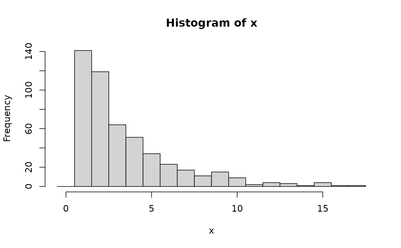
 ## corresponding sample with histogram of empirical frequencies
set.seed(0)
x <- random(X, 500)
hist(x, breaks = -1:max(x) + 0.5)
## corresponding sample with histogram of empirical frequencies
set.seed(0)
x <- random(X, 500)
hist(x, breaks = -1:max(x) + 0.5)