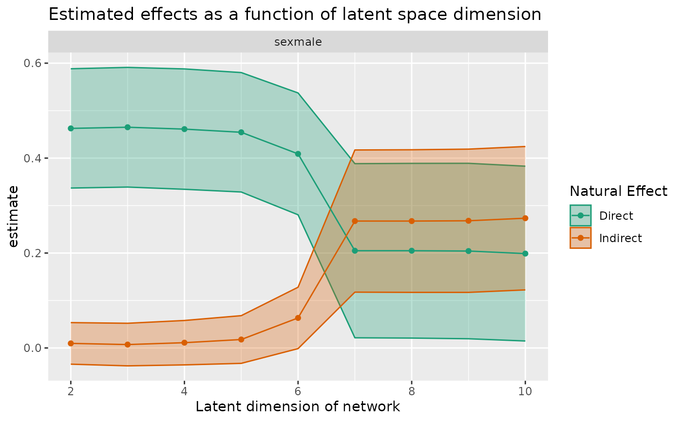
Estimate mediated effects for a variety of embedding dimensions using custom embedding

Usage

sensitivity_curve_custom(graph, formula, X_max, ..., node_data = NULL)

Arguments

graph

A tidygraph::tbl_graph() object.

formula

Details about the nodal design matrix. Of the form outcome ~ nodal_formula. For now, no interactions or fancy stuff are allowed in the formula.

X_max

TODO

...

Arguments passed on to estimatr::lm_robust

data: A data.frame
weights: the bare (unquoted) names of the weights variable in the supplied data.
subset: An optional bare (unquoted) expression specifying a subset of observations to be used.
clusters: An optional bare (unquoted) name of the variable that corresponds to the clusters in the data.
fixed_effects: An optional right-sided formula containing the fixed effects that will be projected out of the data, such as ~ blockID. Do not pass multiple-fixed effects with intersecting groups. Speed gains are greatest for variables with large numbers of groups and when using "HC1" or "stata" standard errors. See 'Details'.
se_type: The sort of standard error sought. If clusters is not specified the options are "HC0", "HC1" (or "stata", the equivalent), "HC2" (default), "HC3", or "classical". If clusters is specified the options are "CR0", "CR2" (default), or "stata". Can also specify "none", which may speed up estimation of the coefficients.
ci: logical. Whether to compute and return p-values and confidence intervals, TRUE by default.
alpha: The significance level, 0.05 by default.
return_vcov: logical. Whether to return the variance-covariance matrix for later usage, TRUE by default.
try_cholesky: logical. Whether to try using a Cholesky decomposition to solve least squares instead of a QR decomposition, FALSE by default. Using a Cholesky decomposition may result in speed gains, but should only be used if users are sure their model is full-rank (i.e., there is no perfect multi-collinearity)

node_data

TODO

Value

A rank_sensitivity_curve object, which is a subclass of a tibble::tibble().

Examples


library(tidygraph)
library(invertiforms)
#> 
#> Attaching package: ‘invertiforms’
#> The following object is masked from ‘package:base’:
#> 
#>     transform

# suppose you want to use the degree-normalized Laplacian embedding
# instead of the adjacency spectral embedding. you can do that as
# follows

data(smoking)

smoking2 <- smoking |>
  mutate(
    smokes_int = as.integer(smokes) - 1
  )

A <- igraph::as_adj(smoking2)

# here we construct our "custom" embeddings

iform <- NormalizedLaplacian(A)
L <- transform(iform, A)

s_max <- RSpectra::svds(L, 10, 10)
X_max <- s_max$u %*% diag(sqrt(s_max$d))

# and now we plug them into the product-of-coefs estimator

curve_custom <- sensitivity_curve_custom(smoking2, smokes_int ~ sex, X_max)
curve_custom
#> # A tibble: 18 × 6
#>    term    estimand estimate conf.low conf.high  rank
#>    <chr>   <chr>       <dbl>    <dbl>     <dbl> <int>
#>  1 sexmale nde       0.463    0.337      0.588      2
#>  2 sexmale nie       0.00964 -0.0341     0.0534     2
#>  3 sexmale nde       0.465    0.339      0.591      3
#>  4 sexmale nie       0.00718 -0.0377     0.0520     3
#>  5 sexmale nde       0.461    0.334      0.588      4
#>  6 sexmale nie       0.0111  -0.0356     0.0579     4
#>  7 sexmale nde       0.454    0.329      0.580      5
#>  8 sexmale nie       0.0178  -0.0324     0.0681     5
#>  9 sexmale nde       0.409    0.281      0.537      6
#> 10 sexmale nie       0.0633  -0.00139    0.128      6
#> 11 sexmale nde       0.205    0.0214     0.388      7
#> 12 sexmale nie       0.267    0.118      0.417      7
#> 13 sexmale nde       0.205    0.0209     0.389      8
#> 14 sexmale nie       0.267    0.117      0.418      8
#> 15 sexmale nde       0.204    0.0194     0.389      9
#> 16 sexmale nie       0.268    0.117      0.419      9
#> 17 sexmale nde       0.199    0.0147     0.383     10
#> 18 sexmale nie       0.273    0.122      0.424     10

plot(curve_custom)